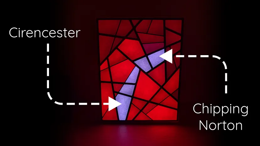
Taking Dijkstra's Shortest Path Through the Cotswolds

A DIY Raspberry Pi Pico and Neopixel LED project

Dec 7, 2024

5 min read

I designed and built an illuminated map of the Cotswolds, a beautiful region in the UK — and also where I happen to live. This unique piece of wall art visualises how computers find the shortest path between locations, bringing two famous algorithms to life with a Raspberry Pi Pico, Neopixel LEDs, and Python code.

My inspiration came from Craig and Dave, popular UK computer science educators. They use a map of Gloucestershire to teach shortest path algorithms, specifically Dijkstra's algorithm to find the quickest route between Stroud and Tewkesbury. Living in Gloucestershire myself, I know this route well and was fascinated by their approach. I decided to expand on their idea and create a more detailed version encompassing the entire Cotswolds.

Designing a Glowing Map

I began with a striking geometric design by Cary Smith, which I discovered on Pinterest.

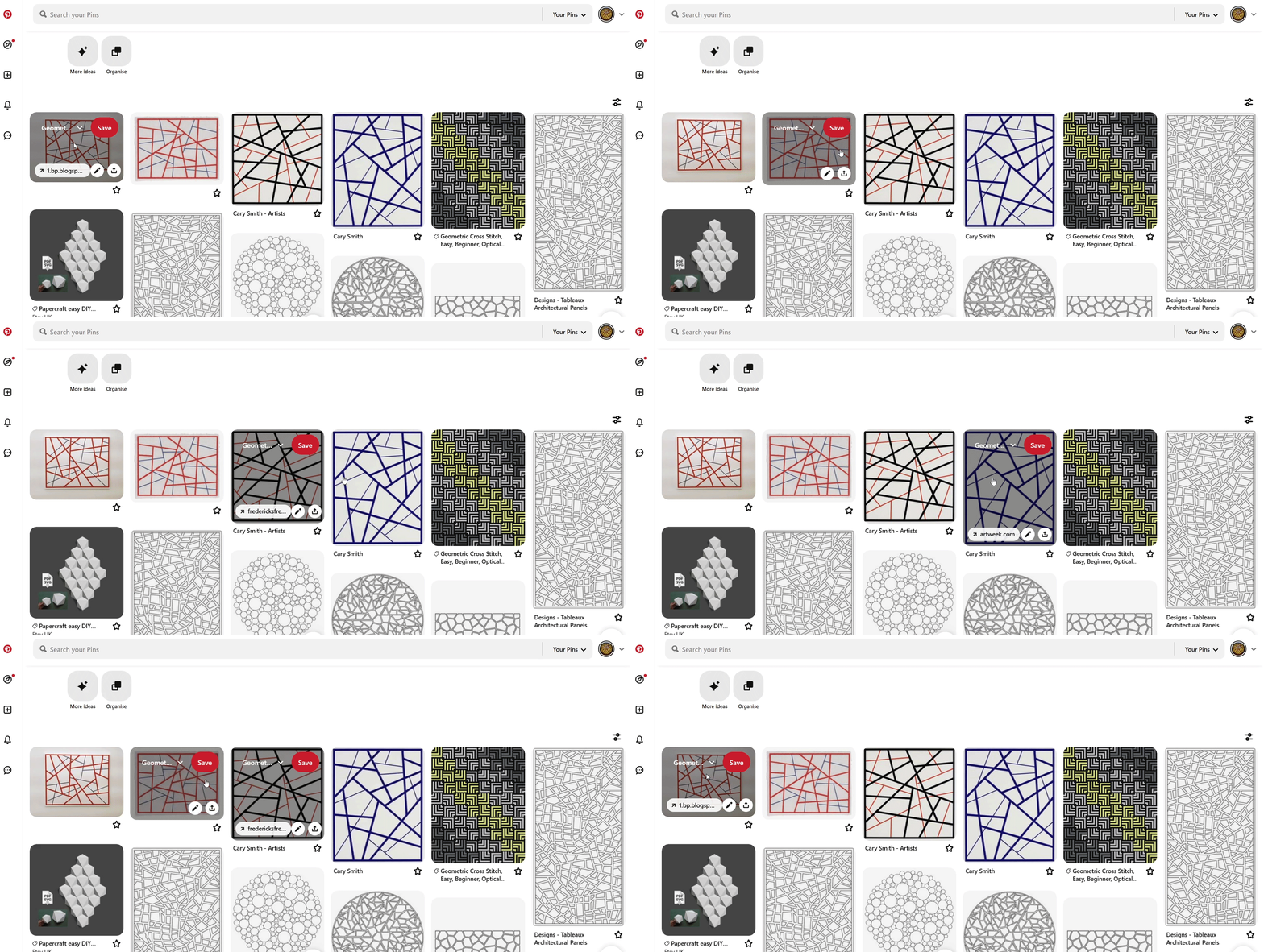
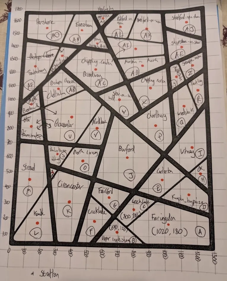
Animated image of Smiths work found on Pinterest — I found Cary Smith's work on Pinterest

Smith's work captures a map-like essence with its asymmetric, straight-lined polygons. I transformed his design into an SVG file with transparent polygons, then overlaid it onto a map of the Cotswolds using OpenMaps and Photoshop. Each polygon now represents a town or village, including Tewkesbury, Evesham, and Stratford-Upon-Avon to the north, and Stroud, Cirencester, Faringdon, and a touch of Oxford to the south.

Hand scribbled towns written on to printout of map — I made a crude grid and labelled towns approximately where they would be found

To bring my design to life, I used a Cricut cutting machine to create two versions: a vinyl sticker for precise LED placement and a mount board cutout for the visible layer.

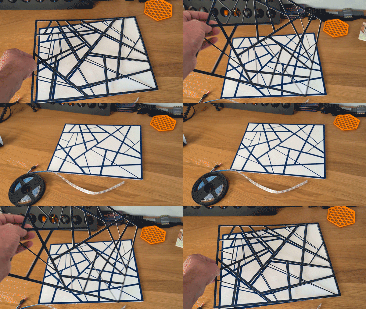
Animation of two versions of the map outline; one vinyl sticker, one mount board

I adhered the vinyl sticker to 5mm foam board and the mount board cutout to a piece of Lutradur fabric from SpunArt. This unique fabric, with its randomly fused polyester fibres, beautifully diffuses the light from the LEDs.

Wiring the Cotswolds

Next, I cut individually addressable Neopixel LED strips to size. Each town received at least one LED, with larger towns accommodating up to eleven.

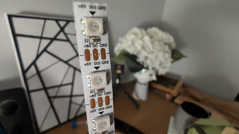
Close up of Neopixel LEDs — Each Neopixel LED is capable of emitting red, green and blue light and can be controlled separately

Thanks to their adhesive backing, attaching the LEDs was straightforward. I threaded the flexible strips through the foam board, using a permanent marker to label connections and ensure correct data and power flow.

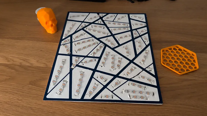
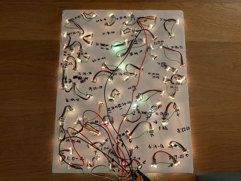
The back of the board showing all the LEDs soldered

After a long soldering session, I successfully connected all 41 towns, totalling 144 LEDs.

To prevent dimming from voltage drop, I incorporated Wago connectors to split and inject power at three points along the LED string.

Close up of Wago connector — Wago connectors allowed for easy splitting of power, preventing voltage drop

Adding Depth and Dimension

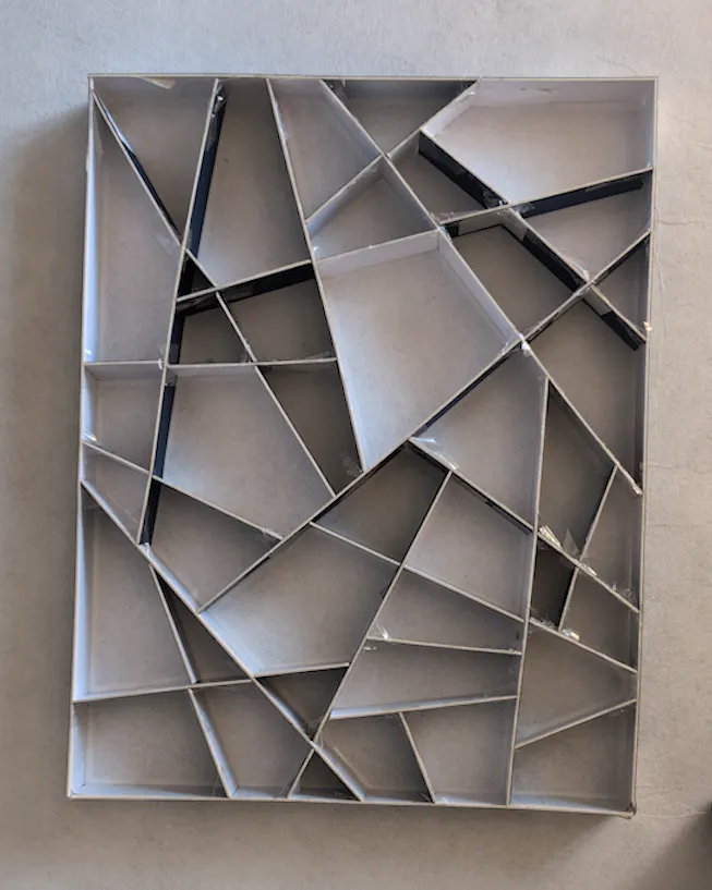
To enhance light diffusion and hide individual LEDs, I constructed a frame from mount board strips. This frame, positioned behind the map outline, effectively prevented light bleed between towns, except, interestingly, between Cheltenham and Gloucester — a quirk that mirrors reality!

The inside of the frame showing partitions

Mapping the Towns

Instead of using precise longitude and latitude, I opted for a simpler approach. I created a grid system, marked the estimated centre of each town with an orange dot, and approximated the x and y coordinates by hand.

Bringing the Map to Life with Code

Initially, I hoped Gemini AI could generate the code for me. While it cheekily suggested I tackle it myself, it did provide a helpful function for calculating the distance between two points using Pythagoras' theorem.

Code snippet for finding distance between points — Python function to find the distance between two points

A Raspberry Pi Pico, programmed with MicroPython, controls the LEDs.

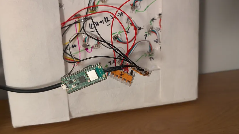
Raspberry Pi Pico W connected host the Python files and controls the lights

I uploaded three files to the Pico: the Neopixel library, a "main.py" file for the main program, and a "cotswold.py" file containing a class definition for town objects. Each town object stores its name, LED list, coordinates, neighbours, and variables for tracking Dijkstra's algorithm's progress.

Witnessing Dijkstra's Algorithm in Action

When I switch on the model, all towns illuminate with a faint red glow. The program then randomly selects two towns as the start and end points for the shortest path demonstration.

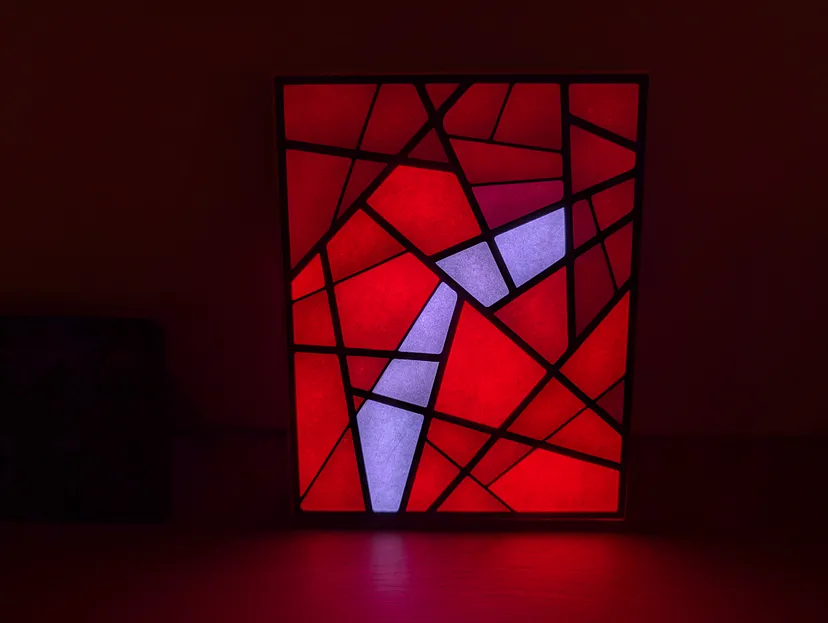
The shortest path between Cirencester and Chipping Norton

Dijkstra's algorithm begins by assuming every town is infinitely far from the starting point (represented by the value 9999). It sets the starting town's distance to 0 and then calculates the straight-line distance to each neighbour. If this calculated distance is shorter than the currently recorded distance for a neighbour, the algorithm updates the neighbour's distance and notes the current town as its "previous town." These neighbours glow bright red to signal the calculation. The algorithm marks the starting town as "visited" and then selects the unvisited neighbour with the shortest distance as the new "current town." This process repeats until it reaches the destination, allowing us to trace the shortest path by following the chain of "previous town" links.

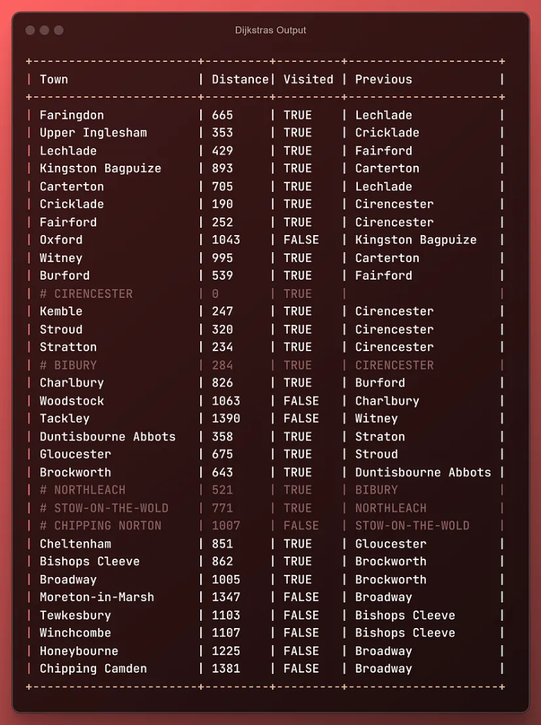
The output of Dijkstra's shortest path between Cirencester and Chipping Norton

Watching the algorithm unfold is mesmerising. It's like witnessing a digital ghost navigate the map, especially in timelapse. At a slower pace, it becomes almost hypnotic, reminiscent of a lava lamp, as you anticipate the next illuminated town.

What's Next?

I plan to implement the A* algorithm, which adds a layer of "common sense" to pathfinding. I also have ideas for visualising other algorithms, so stay tuned!

Thanks for reading!